Statcast Defensive GAM: 2015-2016

Since Statcast data became publicly available in 2015, one of its main uses has been to analyze individual hitters, with exit velocity and launch angle combinations beginning to replace the soft, medium, and hard contact distinctions that previously characterized batted balls. While there’s nothing wrong with knowing exactly how hard Giancarlo Stanton hits his home runs, or even his double play balls, Statcast has the potential to be so much more. By measuring exactly where each defender is on the field prior to each pitch, combined with the batted ball data (i.e. exit velocity and launch angle) that Statcast provides, Statcast has the potential to cut through the noise and/or guess work that traditional advanced defensive statistics like ultimate zone rating (UZR), defensive runs saved (DRS), or park adjusted defensive efficiency (PADE) possess. In doing so Statcast can provide perhaps the most effective measure of a position player’s true defensive talent. Unfortunately, MLB does not yet make any defensive Statcast metrics publicly available (although they’ve provided interesting visuals in this regard). While this means it’s currently not possible to evaluate individual defense performance using only Statcast data, enough publicly available Statcast batted ball data exists to help lay the ground work for the creation of a team-wide Statcast dependent defensive metric to hold fans over until MLB does release additional defensive Statcast data. With that in mind, I set out to create a rudimentary defensive metric (Statcast Defensive Efficiency) to measure an individual MLB team’s defensive ability based on the probability a batter would reach base (i.e. via single, double, triple, home run, fielding error, or fan interference) using the individual Statcast exit velocity and launch angle combinations for each ball in play for both the 2015 and 2016 seasons. To do this I utilized a general additive model (GAM), which has been used a couple of times before in Exploring Baseball with R.

First, let me explain how I compiled the Statcast data. I went to baseballsavant.com and then to the Statcast Search section. From here I entered in the maximum and minimum ranges for launch angle and exit velocity on an individual team-by-team basis for both 2015 and 2016 (60 total CSV files). Please note that there may be a faster way to compile this data, but this was the most efficient way I came up with. After doing this I ended up with a preliminary sample size of 224,266 balls in play between the 2015 and 2016 regular seasons. As Statcast was initially rolled out in 2015, there were some kinks that still needed to be worked in the collection of the batted ball data; to be clear, this data is far from from perfect or complete. To try and combat this I removed all balls in play for 2015 and 2016 that had a listed exit velocity of zero. This brought my total balls in play down from 112,455 to 111,995 in 2015, and 111,811 to 111,809 in 2016. Altogether I ended up with 223,764 balls in play to sample from across the 2015 and 2016 regular seasons.

Next, I created some plots using the GAM that illustrate what combination of exit velocity vs. launch angle typically have higher reach base probabilities for both the 2015 and 2016 seasons.

While the above two graphs give an overall view of what combinations of exit velocity vs. launch angle lead to high reach base probabilities, I’ve synthesized the main ideas in the following plots below. For both the 2015 and 2016 season, I plotted ground balls (zero degree launch angle), line drives (fifteen degrees), and fly balls (thirty degrees) in conjunction with exit velocity vs. reach base probabilities.

The only major difference between the two above graphs is the ground ball reach base probability between twenty five and fifty degrees, which may have occurred due to sample size differences in the 2015 season vs. the 2016 season.

Now that each batted ball in play from my sample has a reach base probability attached to it, I assigned individual credits or debits to each team’s defense. I treated batted ball outs as positives and batted ball reach base events (i.e. errors, hits, fan interference) as negatives. For example, take this catch Kevin Pillar made on Miguel Sano in 2015. Bo Schultz serves up a four seam fastball virtually right down the middle of the plate, and Sano crushes it with an exit velocity of 106.19 mph and a launch angle of 19.82. According the GAM I used, Sano’s batted ball had a probability of reaching base of 0.81. Unfortunately for Sano, Kevin Pillar patrols centerfield for the Blue Jays, and he made a spectacular catch to prevent extra bases. Thus, Pillar’s excellence earns the Blue Jays team Statcast Defensive Efficiency a 0.81 addition. If Sano’s batted ball had fallen in, the blame would lie primarily with Bo Schultz for not executing his pitch, and the Blue Jays Statcast Defensive Efficiency would be deducted only 0.19 (1-0.81). In simplest terms I wanted to create a metric that penalized the defense for failing to make plays it should have made (based on the reach base probabilities derived from the exit velocity and launch angle), but also gave them credit for making outstanding catches, like the Kevin Pillar example referenced above. As such, I assigned each batted ball in play as either a positive or a negative to the individual team defenses, depending on the batted ball outcome (i.e. reach base vs. out) and Statcast data (probability of reaching base based on exit velocity and launch angle combinations). I then totaled the individual team amounts for both the 2015 and 2016 seasons. Finally, like many advanced baseball metrics (including OPS+ and wRC+), I adjusted each year’s results to fit on a one hundred point scale (i.e. 100 is equal to average, 110 is ten percent above average) to create the Statcast Defensive Efficiency metric. Below I’ve listed the Statcast Defensive Efficiency rankings for both the 2015 and 2016 regular seasons:

2015:

Rank	Team	League	Statcast Defensive Efficiency
1	KCA	AL	156.8
2	TBA	AL	153.0
3	CLE	AL	152.4
4	TOR	AL	144.8
5	SFN	NL	144.5
6	MIN	AL	141.6
7	CHN	NL	122.2
8	MIA	NL	120.3
9	TEX	AL	115.1
10	HOU	AL	113.2
11	OAK	AL	111.0
12	BAL	AL	110.8
13	AZN	NL	108.3
14	PIT	NL	101.5
15	STL	NL	93.5
16	CIN	NL	92.2
17	SEA	AL	92.0
18	LAA	AL	90.0
19	WAS	NL	87.9
20	MIL	NL	86.9
21	LAN	NL	86.7
22	NYA	AL	84.7
23	DET	AL	84.7
24	ATL	NL	76.6
25	SDN	NL	71.0
26	NYN	NL	70.5
27	PHI	NL	59.4
28	BOS	AL	52.9
29	CHA	AL	44.5
30	COL	NL	31.0

2016:

Rank	Team	League	Statcast Defensive Efficiency
1	CHN	NL	231.5
2	TOR	AL	175.2
3	SFN	NL	132.9
4	KCA	AL	118.4
5	SEA	AL	118.2
6	BOS	AL	117.7
7	MIA	NL	116.3
8	CLE	AL	115.7
9	TEX	AL	115.3
10	LAN	NL	105.6
11	WAS	NL	105.1
12	ATL	NL	104.1
13	PHI	NL	100.6
14	OAK	AL	98.0
15	LAA	AL	97.8
16	BAL	AL	92.7
17	CIN	NL	87.6
18	CHA	AL	85.5
19	PIT	NL	83.8
20	HOU	AL	83.0
21	SDN	NL	82.7
22	NYA	AL	81.7
23	COL	NL	79.9
24	NYN	NL	77.8
25	DET	AL	75.6
26	STL	NL	73.5
27	MIL	NL	70.5
28	TBA	AL	68.7
29	AZN	NL	59.6
30	MIN	AL	45.1

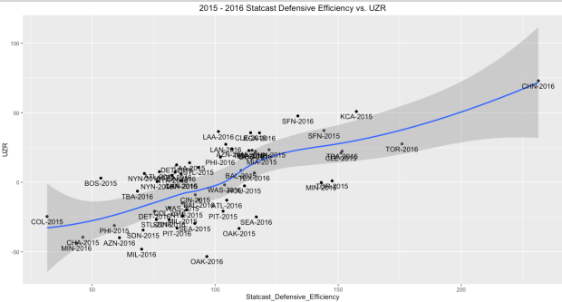
To give more context (and to use as a self check for myself) I’ve added plots that compare the 2015-2016 Statcast Defensive Efficiency I’ve developed (along with correlation coefficient calculations) to three previously mentioned widely used advanced defensive metrics:

• DRS: Correlation coefficient (“r”) = 0.5727
• UZR: r = 0.6926
• PADE: r = 0.6929

A couple of things jumped out at me:

1.) The American League had more teams ranked in the top 10 of Statcast Defensive Efficiency for both seasons. The underlying reason for this is most likely because of the existence of the designated hitter, there are more chances for an American League defense to accumulate positive debits. As a shorthand to support the notion of increased balls in play between the two leagues, since the designated hitter was instituted in 1973, the American League has had a lower strikeout rate than the National League in each season.

2.) Park factors can have a disproportionate effect on an individual team’s Statcast Defensive Efficiency. The Rockies had the lowest Statcast Defensive Efficiency rating in 2015. Whether this is due to their defense being this below average, or whether the metric unfairly penalized the Rockies outfielders for having an inordinate amount of bloop hits fall due to the cavernous dimensions of Coors Field is unclear.

3.) According to Statcast Defensive Efficiency, the 2016 Chicago Cubs were far and away the best defensive team of the past two seasons. This in and of itself isn’t particularly shocking; the 2016 Cubs led MLB in PADE, DRS, and UZR as well, and other analysts (including myself) have examined the 2016 Cubs defense before. What’s shocking is how far ahead the 2016 Cubs are in Statcast Defensive Efficiency. To put it simpler:

• In 2015, the Kansas City Royals led the MLB in Statcast Defensive Efficiency with a score of 156.8. The 2016 Chicago Cubs Statcast Defensive Efficiency was nearly 75 percentage points higher.
• The difference between the 2016 Cubs and the second place team in Statcast Defensive Efficiency (Toronto Blue Jays) was 56.3 percentage points. The difference between the 2015 Kansas City Royals and the 2015 fourteenth place team in Statcast Defensive Efficiency (Pittsburg Pirates) was 55.3 percentage points.
• The difference between the 2016 Cubs and the third place team in Statcast Defensive Efficiency (San Francisco Giants) was 98.6 percentage points. The difference between the 2015 Kansas City Royals and the 2015 twenty-seventh place team in Statcast Defensive Efficiency (Philadelphia Phillies) was 97.4 percentage points.

So the Cubs essentially lapped the Statcast Defensive Efficiency field in 2016, and earned themselves a 109.3 percentage point increase from their corresponding Statcast Defensive Efficiency score in 2015. Just what has changed with the Cubs defense from 2015 vs. 2016? Having watched the Cubs intently over the past two seasons there are three major differences worthy of remark:

1.) After initially working in at second base upon his call up to the majors in June 2015, Addison Russell was the Cubs’ starting shortstop for the entire 2016 season.

2.) Due to strikeout issues and a broken finger, Javier Baez was not recalled to the Cubs major league team until September 2015. Baez appeared in 143 games during the 2016 season, primarily at second and third base.

3.) Jason Heyward, who from 2010-2015, ranked second in the MLB in DRS (behind only Andrelton Simmons, and in front of Alex Gordon, Adrian Beltre, and Co.) was signed in the 2016 offseason, replacing Jorge Soler (he of -8 DRS in 2015) as the Cubs primary right fielder. Heyward was a massive disappointment at the plate in 2016, but his glove work was as excellent as advertised.

Since visuals often speak louder than the written word when talking about defense in baseball, I’ve included some plays for Russell, Baez, and Heyward that show the defensive impact of each.

Russell and Piscotty: Exit Velocity: 91.62 mph , Launch Angle: 6.60 degrees , Reach Base Probability: 0.6758, Contribution to Cubs Statcast Defensive Efficiency: +.6758

Russell, Peralta: Exit Velocity: 90.49 mph , Launch Angle: 6.51 degrees , Reach Base Probability: 0.6253, Contribution to Cubs Statcast Defensive Efficiency: +.6253

Russell, Meyers: Exit Velocity: 109.6 mph , Launch Angle: 6.42 degrees , Reach Base Probability: 0.7256, Contribution to Cubs Statcast Defensive Efficiency: +.7256

Russell, Goldschmidt: Exit Velocity: 91.99 mph , Launch Angle: 10.09 degrees , Reach Base Probability: 0.7367, Contribution to Cubs Statcast Defensive Efficiency: +.7367

Baez, Heyward, Dietrich: Exit Velocity: 110.61 mph , Launch Angle: 9.00 degrees , Reach Base Probability: 0.7789, Contribution to Cubs Statcast Defensive Efficiency: +.7789

Baez, Crawford: Exit Velocity: 65.66 mph , Launch Angle: 19.59 degrees , Reach Base Probability: 0.6978, Contribution to Cubs Statcast Defensive Efficiency: +.6978

Heyward, Schebler: Exit Velocity: 96.85 mph , Launch Angle: 15.66 degrees , Reach Base Probability: 0.6277, Contribution to Cubs Statcast Defensive Efficiency: +.6277

Heyward, Span: Exit Velocity: 103.48 mph , Launch Angle: 29.21 degrees , Reach Base Probability: 0.8846, Contribution to Cubs Statcast Defensive Efficiency: +.8846

What’s more is that the ages of the Russell, Baez, and Heyward trio are 22 years old, 23 years old, and 27 years old respectively. This trio’s youth, combined with the Cubs overall youth and overwhelming versatility, make it likely that their defensive performance during the 2016 season was not a fluke.

To be clear, there are a couple of small fixes that could improve Statcast Defensive Efficiency as currently constructed (i.e. league adjustment, park adjustment, batter handedness adjustment). Still, after watching the 2016 playoffs, it confirms my original belief that no matter what metric is developed, it will be difficult to form a complete assessment of both an individual and team defensive ability based on the data that is currently publicly available, especially without the starting point for each defensive player. Take for instance this play made by Javier Baez in game five of the 2016 NLCS. By all accounts it’s a phenomenal play, given the high leverage point at which it was made (top of the seventh, two run game), the bare hand/arm strength it took to beat Adrian Gonzalez to first base, and the knowledge that Baez was the only player who could make the play because the next closest position player to the ball was Jon Lester (who can’t throw to first base). But the most impressive part of the play is the range that Baez displayed just by getting to the ball. Check out the screenshot below:

Baez was shifted into short right field to guard against the pull tendencies of Gonzalez and still was able to get to a bunted ball in time to throw out the (admittedly slow) runner. In Statcast Defensive Efficiency the above play would simply be treated like any other slow ground ball when it is anything but. Thus, with it’s limitations, it’s best to view Statcast Defensive Efficiency as a component of something bigger, like an appetizer before the main course. But it’s comforting to know that after decades of facing uncertainty when evaluating defense, Statcast data proves that the main course is coming soon.