In an earlier post, I described how one can compute end-of-inning win probabilities for the home team using Retrosheet game log data. One is usually interested in computing win probabilities after each play, and using these to find so-called WPA (win-probability added) values that we can attribute to specific players. Here we describe using Retrosheet play-by-play data to compute these win probabilities and we’ll contrast these values with the ones posted on the Baseball-Reference site.

To review some previous work, we have already described in a previous post the process of downloading all play-by-play data for a specific season from Retrosheet and computing the run values (from the run expectancy table) for all players. We will be using these run values in this work.

Computing the Inning Win Probabilities

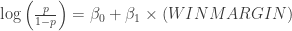
I wrote a new function prob.win.game2.R that will download the Retrosheet play-by-play data for a specific season and use these to estimate the probability the home team wins at the end of each half-inning. Essentially, I collect the winning margin (home score – visitor score) and the ultimate game outcome (1 if the home team wins, and 0 otherwise) at the end of a specific half-inning and fit the logistic model

where p is the probability the home team wins. We fit 16 of these models, corresponding to each of the half-innings top-of-first, bottom-of-first, …, top-of eighth, bottom-of-eighth. (In the 9th inning and beyond, we use the same model that was used for the 8th inning.) For example, at the end of the 4th inning, we have the fit

So by leading by an additional run after 4 innings, the home team’s probability of winning (on the logit scale) is increased by 0.632.

Computing the Play Win Probabilities

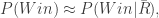
Actually, we want to compute the probability the home team wins after each play in an inning. For example, suppose the home team has runners on 1st and 2nd with one out in the 4th — what is the probability they will win? Using a rule of probabilities

where is the probability the team scores R runs in the inning, and is the probability the team wins at the end of the inning if they have scored R runs. This probability is tedious to compute, but we can approximate it by

where is the expected run value, and is the probability the home team wins (computed using the logistic model) if the team has scored runs. For example, suppose that a home team currently has a 2 run lead, and runners on 1st and 2nd with two outs in the bottom of the forth. The expected number of runs in the remainder of the inning is 0.40 (from 2014 data). Using the logistic model, the logit of the probability of the home team winning at the bottom of that inning is estimated to be

and the probability the home team wins the game is exp(1.59) / (1 + exp(1.59)) = 0.83.

To compute these win probs, I first use the function compute.runs.expectancy to compute all of the run values and then use a new function compute.win.probs to compute the win probabilities after all plays. This last function uses both the data frame that contains the Retrosheet data and run values, and also the data frame containing the logistic regression coefficients for all half-innings.

Displaying Play Win Probabilities

I have saved the data frame containing all of this work for the 2014 season on my website. You can plot the win probabilities for a specific game by downloading the data frame and sourcing in a new function graph.game that will do the plotting. The function outputs the rows of the data frame corresponding to the game. Here is an illustration of how it works — we’ll plot the win probabilities for the New York Yankees at Tampa Bay Rays game of April 18, 2014.  The plays

load(url("http://bayes.bgsu.edu/baseball/pbp2014winprob.Rdata"))
library(devtools)
source_gist("a8e5255c98954d151974")
d.game <- graph.game(d, "TBA201404180")

You can plot win probabilities for any game for the 2014 season — just change the game code in the input of graph.game .

Checking My Work

If you look at the Baseball-Reference description of this game here, you’ll see the same type of win probabilities plotted and each play has an associated value of WPA. I’m not sure of the exact method that was used, but it is easy to download their data and compare their values of WPA with my values. Here is a scatterplot of the two sets of values for this particular game.

I’m encouraged that the WPA values are similar in this case. In particular, both methods would identify the important plays in this game. The key play was James Loney’s single in the bottom of the 7th that raised the Tampa win probability by over 40%.

The code for the two new functions prob.win.game2.R and compute.win.probs can be found on my gist site here.