One of my fun units in my data science class is mapping. I wanted to show the relative ease of creating region maps colored with an interesting measurement for each region. This post will demonstrate scraping several datasets from html tables, getting map data using the mapdata package, merging this map data with the data frame of measurements, and constructing the map using the ggplot2 package.

A Question and Relevant Data

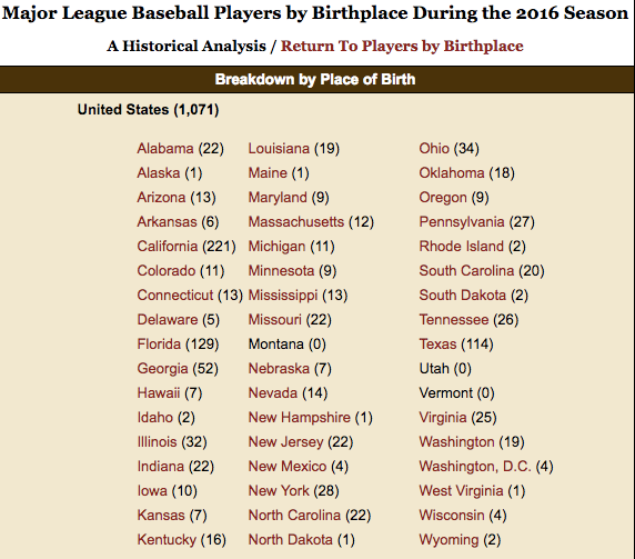
I am wondering about the locations of the birthplaces of the American players who played in the current MLB season. Doing a little searching, I found this page from Baseball Almanac that displays the number of players born in each state:

Scraping the Data

Using the readHTMLTable function in the XML package, I read this html page into R.

 
library(XML)
d <- readHTMLTable("http://www.baseball-almanac.com/players/birthplace.php?y=2016")

Some Data Cleaning

Below, I pick out the list element containing the table, choose the relevant rows and columns, convert each column to character type, and make a long vector of values.

 
d1 <- d[[1]][14:30, 2:4]
for (j in 1:3)
  d1[, j] <- as.character(d1[, j])
d1 <- unlist(d1)

A typical value in my vector is “Alabama (22)”. I want to extract the number from each string in my vector. (I use the str_extract function in the stringr package.) The completed list of counts is stored in values .

 
library(stringr)
values <- as.numeric(str_extract(d1, '[0-9]+'))

Similarly I want to extract the state names — all of the names will be in the vector state_names .

 
state_names <- str_extract(d1, '[a-zA-z ]+')

I remove the District of Columbia data from each vector.

 
values <- values[-48]
state_names <- state_names[-48]

I create a data frame with two variables State and N_Player .

 
final <- data.frame(State=state_names, 
                    N_Player=as.numeric(values))

Collecting State Populations

The raw number of players in a state should be standardized by, say the state’s population. So I want to collect current state populations. I find a Wikipedia page with the data and read it in R by the htmltab function in the htmltab package.

 
library(htmltab)
p <- htmltab("https://en.wikipedia.org/wiki/List_of_U.S._states_and_territories_by_population")

More Cleaning

I do some cleaning of this data frame. I select the rows corresponding to the 50 states, use shorter variable names, and remove the commas from the population values, and convert the results to numeric type.

 
p <- p[c(1:29, 31:49, 51:52), 3:4]
names(p) <- c("State", "Population")
p$Population <- as.numeric(str_replace_all(p$Population, ",", ""))

Merging the Two Datasets

Okay, now I merge the baseball data with the population data using the inner_join package.

 
library(dplyr)
final_data <- inner_join(final, p)

I create a density variable Pct_MLB which divides the number of players by the corresponding state’s population and make it a percentage.

 
final_data <- mutate(final_data, 
                     Pct_MLB = 100 * N_Player / Population,
                     state=tolower(State))

Merging with Mapping Data

I collect the map data for the United States using the map_data function in the mapdata package. Then I merge this mapping data with my measurement data using another application of inner_join .

 
library(mapdata)
states <- map_data("state")
states <- inner_join(states, final_data, by=c("region"="state"))

Ready to Graph

I am ready to graph using ggplot2 . I use geom_polygon with the fill variable is Pct_MLB . I choose a color range of yellow (low) to red (high) so the states are clearly distinguished.

 
library(ggplot2)
ggplot(data = states) + 
  geom_polygon(aes(x = long, y = lat, 
          fill = Pct_MLB, group = group), color = "white") + 
  coord_fixed(1.3) +
  scale_fill_gradient(low = "yellow", high = "red") +
  ggtitle("Density of 2016 MLB Players by State")

As expected, we see a high density of baseball players born in California and Florida. But there are a number of other states with “larger” densities of baseball players such as Texas, Georgia, Oklahoma, and some of the midwestern states. By adjusting by the population sizes, I think this display is perhaps more meaningful that simply scanning a table of number of players from each state.

If you want to try this out, all of the code above can be found as a single chunk on my gist site.