Downloading Retrosheet Data

I recently noticed that play-by-play data for the 2016 season is now available on Retrosheet.  A few years ago, I wrote a post providing functions parse.retrosheet2.pbp and compute.runs.expectancy that help in downloading the data and computing the run values for all plays in a season.  If you follow those instructions, the functions work fine in downloading the 2016 play-by-play data.  After downloading, I save the dataset in a R workspace for future work.

Exploring Stolen Base Attempts

I have always been a bit fascinated with stolen base data.  Why?  Well, teams have varying opinions about the usefulness of this strategy — some teams rarely try to steal and other teams try to steal a lot, and some exploration of SB/CS data might help to explain why.  There are two issues — one is how often do teams attempt to steal?  And second, what is the SB success rate?  I’ll focus on using the Retrosheet data to explore the runner/base situations when teams are more likely to attempt to steal and where they are more successful in stealing.

Working with Retrosheet Data

One has to be a little careful in extracting all of the stolen base information from the Retrosheet play-by-play dataset.  If you look at the EVENT_CD variable, there are codes for SB and CS, but this variable is not helpful if there are multiple events such as a SO and a SB on a single plate appearance — in this case, the EVENT_CD variable indicates a SO and ignores the SB.  One needs to use the EVENT_TX variable that describes all the events for a single play — this variable will catch, for example, two stolen base attempts on a single play.

When one filters the data to include only the plays with SB attempts, it is good to check the work with another data source if possible.  On the Baseball Reference page, I see that there were a total of 2537 SB and 1001 CS which should agree with my work.  (For some reason, I only found 1000 caught stealing, so there is one elusive CS missing from my analysis.)

Success in Attempted SB in Different Situations?

We know that the overall success rate in stealing bases is approximately 100 2537 / (2537 + 1001) = 72 %.  But how does that success rate vary by which base is stolen (2nd or 3rd) and by the runners on base / outs situation?  We first look at attempted steals of 2nd base — the below graph shows the success rate for each situation where the size of the plotting point corresponds to the number of attempts.

The graph tells us that the success rate is approximately 70% when there is only a runner on 1st, but is much higher (over 90%) when there are two runners on base.  It is interesting that the success rate with one runner is highest with 2 out, and it is most difficult to steal 2nd when there is a single out.

What about attempts to steal 3rd base?

It is easiest to steal 3rd base with a single runner and 2 outs — it is hardest to steal with one out.

Team SB Attempts and Success Rates?

We all know there is much variability in team SB attempts.  But I thought it would be interesting to look at the relationship between a team’s attempts and their success rate.

There is a positive association.  Teams that rarely steal (think Baltimore and St. Louis) also have success rates under 60%.  In contrast, teams like Milwaukee and Cincinnati that like to steal also tend to be more successful.  This makes sense — if a team likes to try to steal, they would go to extra effort to be successful at doing it.

Runs Values of Stealing Attempts?

Here I focus on the plate appearances with only a SB attempt and look at the runs value of those attempts.  It would be not meaningful to look at PA where several events like a SO and SB occurred, then the two events would be confounded in the runs value calculation.  I use a violin plot — the red lines correspond to CS and the blue lines to SB.

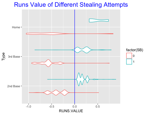
Obviously, run values are positive for SB and negative for CS.  But an attempted steal of 3rd appears to be more risky than an attempted steal at 2nd, since the size of the run values are larger for CS.  As one would expect, the riskiest attempt is home, which makes it one of most exciting plays in baseball.

Quantifying this effect

Below I show the mean, median, and quartile spread (QS) of the run values of attempted steals of 2nd, 3rd, and home. Interesting, the mean runs value of an attempted steal of 2nd base is approximately zero, but the median runs value is 0.092.  The average runs value of an attempted steal of 3rd is smaller than the average for an attempted steal of 2nd base, no matter if you use a median or a mean.  This also demonstrates that an attempt at stealing 3rd base is riskier than an attempted steal of 2nd, since it has a larger quartile spread.

Takeaway from a Team’s Perspective

If you are working for a team, do you care about this analysis?  Well, a team has to make a decision whether to attempt to steal, and obviously if one attempts to steal, they want to be successful.  What factors are relevant in this decision?  A team would think about ..

• who is trying to steal the base?
• who is pitching and catching?
• what is the game situation (runners on base, number of outs, inning, game score)

This brief analysis is a first step, but I’d like to think that the analytics department would look more carefully at the effect the identity of the runner and pitcher and game situation would have on SB attempts and success rates, and use this information to advise the coaching staff.

R Code

As usual, I have posted all of the R code on my GitHub gist site.  This includes the few lines to download the 2016 Retrosheet data and the script to produce this graphs.