Predicting Home Runs from Distance and Spray Angle

Introduction

Over recent years I have spent some time modeling the probability of a home run from the hitter’s launch angle and exit velocity measurements. (We discuss this modeling in the home run chapter in the new edition of ABDWR3e that can be found here.). This model is helpful for understanding the carry properties of the baseball during the Statcast era. The launch angle and exit velocity measurements are strongly related to the distance traveled, but certainly the direction of the hit, that is, the spray angle, plays an important role in home run hitting. (A 350 foot drive down the line is much more likely to be a home run than a 350 foot drive to dead center.). I thought it would be an interesting exercise to illustrate the application of several models for predicting home run hitting based on distance and spray angle. I discuss several popular regression functions in R and illustrate how Bayesian check models by means of simulations from the posterior predictive distribution.

The Data

I collected Statcast data for the 2024 games through April 5. I focus on the balls put into play. Using the events variable, I create a HR variable that is equal to 1 if events = "home_run" and 0 otherwise. The variable hit_distance_sc measures the distance traveled and using the hc_x, hc_y variables, I compute a spray angle variable that falls between -50 and 50 degrees. I focus on only the in-play data where the distance exceeds 300 feet.

A Logistic Model

Certainly the chance of a home run will increase as a function of the distance traveled. Also it is clear that for a given distance, it is more likely to hit home runs for extreme spray angles close to -50 and 50. If p is the probability of a home run, the above discussion motivates the fit of the logistic model where I add spray angle as a quadratic term.

log(p / (1 – p)) = distance + spray_angle + spray_angle^2

I can fit this model in R using the glm() function — by using the family = binomial argument, we are fitting a logistic model on the binary HR response.

lm_fit <- glm(HR ~ hit_distance_sc + spray_angle + 
                                I(spray_angle ^ 2), 
                family = binomial,
                data = sc_ip_300)

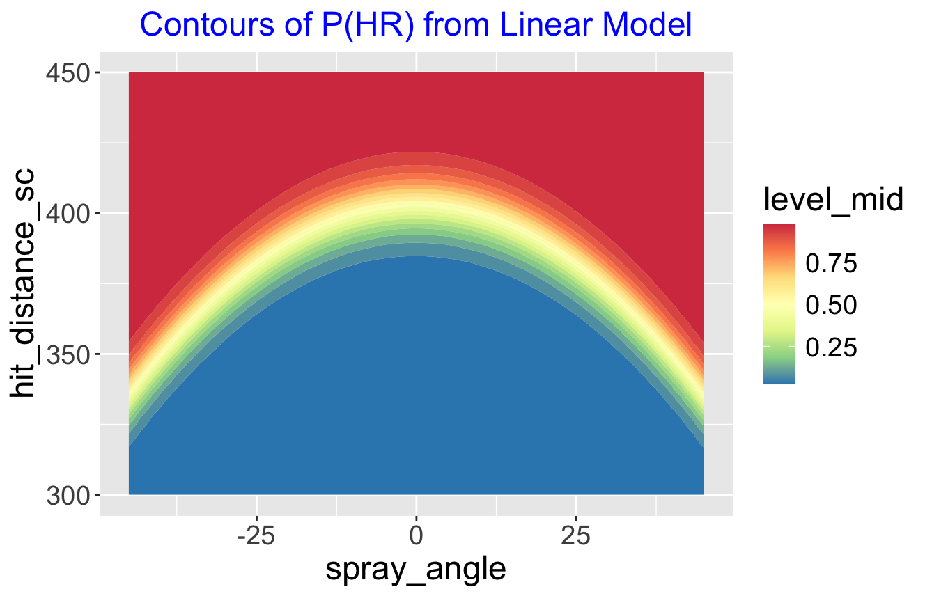
To display the fit, I create a grid of values of distance and spray angle, predict the probability of home run for all values on the grid, and display the fitted probabilities using a contour graph. The filled contour graph is shown below. The yellow region represents the region where the probability of a home run is approximately 0.5. (By the way, this graph reminds us that today (April 8) is a special day where a region of the United States including my city can see the solar eclipse.). On first glance, this looks reasonable and shows the importance of spray angle in home run hitting. The chance of hitting a home run on a 330 foot drive down the third base line is approximately equal to the chance of hitting a home run on a 400 foot drive dead center.

Predictive Check

To check this model, I implement a predictive checking strategy. I look at the observed data and look for interesting features that may not be predicted well from my fitted model. I divide the data into subregions by spray angle and count the number of balls in play and home runs in each region — here’s a table of the counts. To read this table, look at the first row. When the spray angle is between -50 and -45 degrees, there were 11 balls in play and 3 of these balls were home runs.

       SA  0  1
 (-50,-45] 11  3
 (-45,-40] 16 16
 (-40,-35] 24 23
 (-35,-30] 36 20
 (-30,-25] 38 16
 (-25,-20] 61 23
 (-20,-15] 42  9
 (-15,-10] 50  9
  (-10,-5] 81 10
    (-5,0] 65  2
     (0,5] 69  4
    (5,10] 59  6
   (10,15] 62 10
   (15,20] 60 14
   (20,25] 45 12
   (25,30] 51 11
   (30,35] 46 17
   (35,40] 26 10
   (40,45] 28  6
   (45,50]  9  7

I note that there appears to be a large number of home runs hit for negative spray angles (left side of the field) and relative small numbers for positive spray angles. Due to this variation, perhaps the standard deviation of the home run counts might be a reasonable checking function.

Here’s how I implemented my predictive checking. I simulate parameter values from the posterior of my fitted model, and then simulate home run counts from the simulated probabilities. I compute the standard deviation of the simulated HR counts (my checking function). I repeat this method 1000 times and obtain the predictive distribution of my checking function. Here’s a histogram of the predictive distribution of the standard deviation and overlay the observed standard deviation.

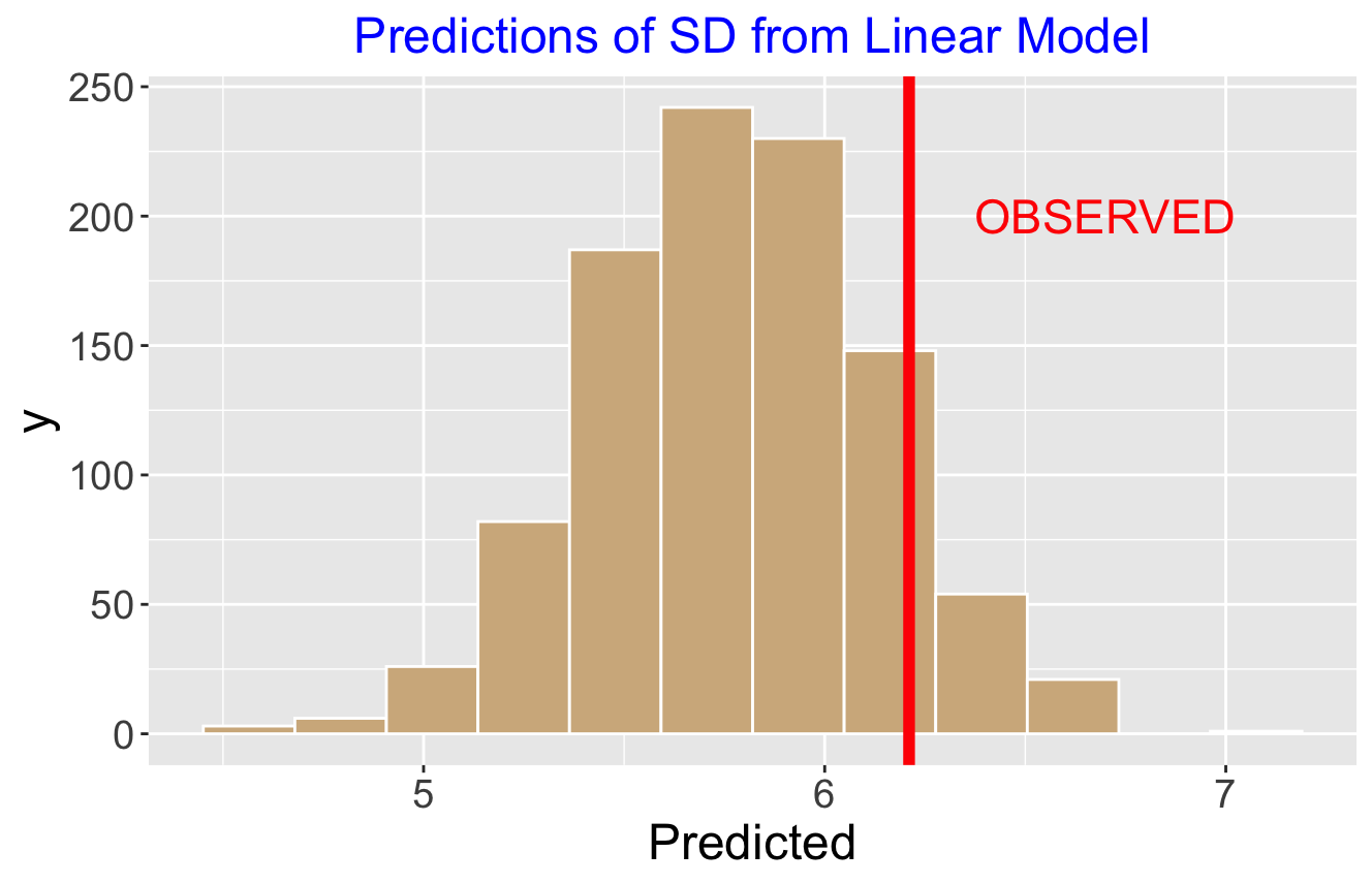
The histogram represents the standard deviations I would predict from our model. The observed standard deviation is in the right tail of the predictive distribution — the chance that the predictive standard deviation is larger than what I observed is about 10%. Since this tail probability is relatively small, that indicates that some misfit of my logistic model — predictions from the fitted model don’t look like what I observed in the data.

A GAM Model

Maybe my choice of a quadratic function for spray angle can be improved. That motives the consideration of a generalized additive model where the logit of the HR probability is a function of the distance plus a smooth function of spray angle. I fit this model by use of the gam() function from the mgcv package

gam_fit <- gam(HR ~ hit_distance_sc + s(spray_angle), 
                family = binomial,
                data = sc_ip_300)

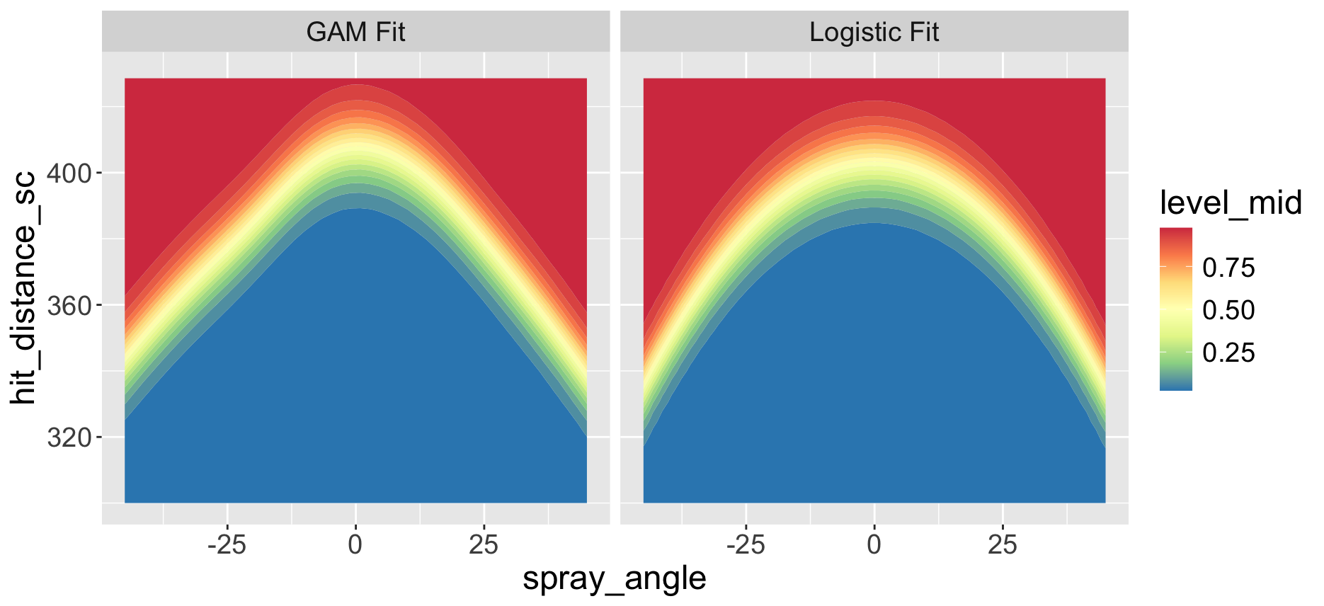
How does this GAM fit compare to the logistic fit? I display contour plots of the fitted probabilities below. The two contour plots look similar, but the GAM fit is more peaked near a spray angle of 0. Perhaps the shape of the contour lines of the GAM fit resemble a typical shape of the outfield fences?

To check the GAM model, I implemented a similar predictive check using the same simulation method with the same standard deviation checking function. In this case the observed SD was more consistent with predictions of the SD from the GAM model. Of course, my model checking activity was limited — I may have found some misfit of this GAM model by using a different checking function.

Remarks

• (Predictive checking?) The predictive checking method is very general, but its success of this method depends on the choice of a suitable checking function. Maybe my particular choice of checking function is lame, but this choice illustrates the checking method.
• (Other useful inputs?). Certainly other inputs may be helpful in predicting home runs. There are ballpark effects, for example, but I don’t think we could pick this up from the limited 2024 data.
• (Got R code?). On my Github Gist site, I include a R script of all of the work for this post.
• (Is the 2024 ball juiced?). I’m not sure if MLB is currently worried about ball effects among all of the issues facing MLB (the latest concern is the rash of pitcher injuries). It is a bit early to see if the carry properties of the ball are similar to those in 2023. When we have several months of data, it will be interesting to see how home run hitting compares to previous Statcast seasons.