Review of the Prediction Problem

Here’s a quick summary of the home run prediction problem described in last week’s post. It is July 1 during a particular season and one is interested in predicting the home run rates for all players in the remainder of the season. One has two sources of information — one has the home run rates for the players in the first half of the season, and one also has the cumulative home run rates for these same players for the previous four MLB seasons. The question is how to best use the two types of information (current and past) if the goal is to predict the second half of the season home run rates.

In last week’s post, I took an empirical approach to this problem and considered the predictive performance of five estimates (just use the current first-half season stats, just use the historical stats, use some weighted average of the current and historical stats where I considered mixing fractions of 0.25/0.75, 0.50/0.50 and 0.75/0.25). By looking at the performance of these estimates over 19 seasons, we learned that it is best to use some weighting of the current and past statistics, perhaps putting heavier weight on the historical home run rates.

Here I illustrate perhaps a simpler Bayesian way of approaching this prediction problem. I place a multilevel model on the home run rates where one assumes that the home run probabilities follow a logistic model where the logit of a probability follows a linear regression model with the logit of the historical home run rate as a covariate. This is a varying intercepts / varying slopes multilevel model where one assumes that each player has a regression with a unique intercept and unique slope. The collection of (intercepts, slopes) for the players follow a bivariate normal model with unknown parameters.

In this post, I’ll introduce this multilevel model, explain how the model is fit using the JAGS software, and see how well these Bayesian estimates perform compared to the estimates described in the previous post. (Of course, these Bayesian estimates will perform well, otherwise I wouldn’t write this post.)

The Multilevel Model

Let denote the home run probability for the th player during the current season. We observe home runs in PAs in the first half the season and we also have , the logit of the observed home run rate of the player in the previous four seasons. The basic model says that is binomial() where the home run probability satisfies the logistic model

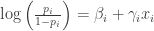
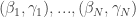
Each hitter has two parameters that describes the regression. We assume that the pairs for the players follow a bivariate normal distribution with mean vector and variance-covariance matrix . We complete the Bayesian model by assigning weakly informative priors on .

Fitting the Model

I use the JAGS software to fit this multilevel Bayesian model by Markov chain Monte Carlo (MCMC). One first defines the model by means of a script, puts the data into a R list, and executes the run.jags() function from the runjags package to take a simulated sample of parameters from the posterior distribution. In particular, one obtains simulated samples of for all players. One can summarize these samples by computation of posterior means, and these means give estimates of which are our Bayesian predictions at the home run rates in the second half of the season.

How Do The Estimates Perform?

I consider a collection of 40 current seasons in this evaluation of methods. For each of these 40 seasons, I predict the second-half season home run rates from the first-half HR rates and the cumulative historical HR rates from the previous four seasons. I compute each of the five empirical estimates (Current, Mix.20, Mix.50, Mix.80, Old) and estimates from the Bayesian multilevel model. For each method, I compute the average absolute prediction error. In the following figure, each small panel compares the predictive performance of the five empirical methods for a given season using connected points and shows the performance of the Bayes multilevel estimate by a horizontal brown line. From looking at this display, we see that the predictive performance of the Bayes estimates is similar to the performance of the Mix.50 and Mix.80 methods which put respectively equal and heavy weights on the historical rates. The Current and Mix.20 (which places heavy weight on Current) methods perform poorly compared with the other methods.

Another way to compare these estimates is to run a prediction contest — for a given season, which method (among the six methods) has the best (lowest) prediction error? For the 40 seasons …

• the Mix.80 method was best for 16 seasons
• the Bayes method was best for 14 seasons
• the Mix.50 method was best for 9 seasons

If we are interested in the worst method with respect to prediction, using the Current home run rates was worst for 36 of 40 seasons. The takeaway is the Bayes multilevel estimates perform well compared to the Mix.80 and Mix.50 methods.

Comments

• Simple method? In the introduction, I described this Bayesian modeling method as “simpler” than the empirical prediction methods described in the last post. Tom Tango has good intuition on suitable predictors since he is very familiar with baseball and has some experience with this particular prediction problem. In contrast, this Bayesian model is straightforward to apply even for those who have limited knowledge of baseball. The fits from the Bayesian model are adaptive in the sense that the data is used to decide how to properly combine the current season and historical data.
• Advantage of Bayes. Although I focused on point prediction of future home run rates, the Bayesian machinery provides a full posterior distribution of all unknowns which can be used for other inferential and prediction tasks. It would be easy, for example, to provide 90% prediction intervals for these future home run rates.
• Other ways to fit multilevel models. There are other ways of fitting these multilevel models. The glmer() function in the lme4 package provides a maximum likelihood fit of a multilevel model and the Stan software provides an alternative MCMC fit of the Bayesian models. I have illustrated the use of the lme4 package in previous posts. For example, this post gives an example of using the glmer() function to fit a varying-intercepts multilevel model for swing rates.
• R code? All of the R functions for this work can be found on my Github Gist site. The get_hr_data() function obtains the home run data, the multilevel_reg() function implements the Bayes fitting using JAGS and the run_and_evaluate() function computes the prediction errors using the six methods.