One of the best known player forecasting systems is Tom Tango’s MARCEL. One of MARCEL’s primary benefits is that it is relatively simple to understand. The basic idea is to take a time-weighted three-year average of past performance and adjust for age. This simple projection system has proven to be relatively robust, in that many others have tried and failed to best MARCEL’s projections. Today, we’ll calculate MARCEL in R.
Being a relatively simple projection system, MARCEL does not require play-by-play data. Thus, we can compute in R using the venerable Lahman Database, which is packaged into R by Michael Friendly. The Lahman Database contains seasonal totals for all major league players going all the way back to 1871.
require(Lahman)
Part of this exercise will involve confirming that we have done the calculations correctly by comparing our results to Tango’s. In his original instructions, Tango computes MARCEL for 2004, so that is the year that we’ll use here. You can easily modify this code to compute MARCEL for any other year.
pred.year = 2004
Building a Data Set
First, we’ll collect the relevant batting statistics for 2001 through 2003, and add a new variable for plate appearances.
B = subset(Batting, yearID >= pred.year - 3 & yearID < pred.year)
B = transform(B, PA = AB + BB + HBP + SF + SH)
We also need to aggregate the statistics by player and year. This will only affect players who played for more than one team in a particular season. We’ll do this for all of the statistics that Tango projects.
require(plyr)
stats = c("PA", "AB", "R", "H", "X2B", "X3B", "HR", "RBI", "SB", "CS", "BB", "SO", "IBB", "HBP", "SH", "SF", "GIDP")
B = ddply(B[, c("playerID", "yearID", stats)], ~playerID + yearID, summarise
             , PA = sum(PA), AB = sum(AB), R = sum(R)
           , H = sum(H), X2B = sum(X2B), X3B = sum(X3B), HR = sum(HR)
           , RBI = sum(RBI), SB = sum(SB), CS = sum(CS), BB = sum(BB)
           , SO = sum(SO), IBB = sum(IBB), HBP = sum(HBP), SH = sum(SH)
           , SF = sum(SF), GIDP = sum(GIDP)
           )
Now, I’ll be following Tango’s instructions in a somewhat different order, and furthermore, I’ll show that the computation of MARCEL can be cast entirely in terms of linear algebra.
In comment #25, Tango walks through an example of how MARCEL computes Carlos Beltran’s home run projection. Let’s follow this example. Beltran hit 24, 29, and 26 home runs in the three years prior to 2004. If we let 
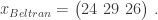
x = subset(B, playerID == "beltrca01")$HR
x
## [1] 24 29 26
Similarly, let 
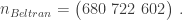
n = subset(B, playerID == "beltrca01")$PA
n
## [1] 680 722 602
The pointwise ratio of these two provides a vector of probabilities (e.g. rate stats) 
Now, we have that


In many forecasting domains, more recent information is considered more valuable. MARCEL incorporates this notion by weighting statistics over time. The season immediately preceding the current one is given a weight of 5, the season before that a 4, and the season two before a 3. Let’s call this vector
and note that it is constant across all players. For the purposes of computation, we also want to add this to our data frame.

B$t = with(B, ifelse(pred.year - yearID == 1, 5, ifelse(pred.year - yearID == 2, 4, 3)))
Thus, Beltran’s time-weighted home run totals is an easy inner product:
t = subset(B, playerID == "beltrca01")$t
t
## [1] 3 4 5
t %*% x
##      [,1]
## [1,]  318
This is the exact calculation that Tango goes through in comment #25.
Computing League Averages
Next, we want to control for the effect of pitchers hitting, so we’ll remove them from our batting statistics before we compute the league averages. To do this, we merge the batting statistics with the pitching statistics, and then restrict our dataset to those players with more plate appearances than batters faced. This seems like a reasonable definition of position players.
P = subset(Pitching, yearID >= pred.year - 3 & yearID < pred.year)
B.pos = subset(merge(x=B, y=P[, c("playerID", "yearID", "BFP")], by=c("playerID", "yearID"), all.x=TRUE), PA > BFP | is.na(BFP))
The league averages can then be computed for the position player statistics by simply summing over all the rows. Let 
p0 = ddply(B.pos, ~yearID, summarise, lgPA = sum(PA), lgAB = sum(AB)/sum(PA), lgR = sum(R)/sum(PA)
           , lgH = sum(H)/sum(PA), lgX2B = sum(X2B)/sum(PA), lgX3B = sum(X3B)/sum(PA), lgHR = sum(HR)/sum(PA)
           , lgRBI = sum(RBI)/sum(PA), lgSB = sum(SB)/sum(PA), lgCS = sum(CS)/sum(PA), lgBB = sum(BB)/sum(PA)
           , lgSO = sum(SO)/sum(PA), lgIBB = sum(IBB)/sum(PA), lgHBP = sum(HBP)/sum(PA), lgSH = sum(SH)/sum(PA)
           , lgSF = sum(SF)/sum(PA), lgGIDP = sum(GIDP)/sum(PA)
           )
p0[, c("yearID", "lgHR")]
##   yearID    lgHR
## 1   2001 0.03003
## 2   2002 0.02787
## 3   2003 0.02854
These numbers match Tango’s.
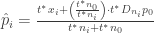
Now, if you follow the description of MARCEL carefully, the estimate of player 

Setting 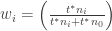

This is simply a weighted average of the player’s rate stats and the league’s rate stats, with the weights 

In practice (the way Tango calculates it), this simplifies to
Note that this generalizes to any number of stats 


Performing the Computation in R
We have computed the league averages, but they need to be linked to the individual batting lines for each player in each season.
M = merge(x=B, y=p0, by="yearID")
Using the matrix equation above and R, we can compute the MARCEL projections for all players at once. The list of statistics that get projected is:
stats.lg = paste("lg", stats, sep="")
Instead of a 

X = M[, stats]
Similarly, the league averages can be expanded as a matrix 
P0 = M[, stats.lg]
Now, we just carry out the matrix computations in the large equation above. First, we compute the quantities needed as columns.
t.X = M$t * X
t.n = M$t * M$PA
t.n0 = M$t * 100
t.P0 = M$t * M$PA * P0
Before we aggregate these columns by player, we’ll add Tango’s estimate for each player’s plate appearance projection.
mPA = with(M, ifelse(pred.year - yearID == 1, 0.5 * PA, ifelse(pred.year - yearID == 2, 0.1 * PA, 200)))
Next, we add these to our data frame and aggregate it by player.
Q = cbind(M[, c("playerID", "yearID")], t.n, t.X, t.n0, t.P0, mPA)

res = ddply(Q, ~playerID, summarise, numSeasons = length(t.n), reliability = sum(t.n)/(sum(t.n) + sum(t.n0))
            , tn = sum(t.n)
            , PA = sum(PA), lgPA = sum(lgPA), mPA = sum(mPA)
            , AB = sum(AB), lgAB = sum(lgAB), R = sum(R), lgR = sum(lgR)
            , H = sum(H), lgH = sum(lgH), X2B = sum(X2B), lgX2B = sum(lgX2B)
            , X3B = sum(X3B), lgX3B = sum(lgX3B), HR = sum(HR),  lgHR = sum(lgHR)
            , RBI = sum(RBI), lgRBI = sum(lgRBI), SB = sum(SB),  lgSB = sum(lgSB)
            , CS = sum(CS), lgCS = sum(lgCS), BB = sum(BB),  lgBB = sum(lgBB)
            , SO = sum(SO), lgSO = sum(lgSO), IBB = sum(IBB),  lgIBB = sum(lgIBB)
            , HBP = sum(HBP), lgHBP = sum(lgHBP), SH = sum(SH),  lgSH = sum(lgSH)
            , SF = sum(SF), lgSF = sum(lgSF), GIDP = sum(GIDP),  lgGIDP = sum(lgGIDP))
The MARCEL projectiions are then the weighted averages of the player’s stats and the league averages, with the weights given by the reliability.
stats.proj = setdiff(stats, "PA")
stats.m = paste("m", stats.proj, sep="")
stats.lg.proj = paste("lg", stats.proj, sep="")
res[, stats.m] = with(res, (reliability * res[, stats.proj]) / tn + (1 - reliability) * res[, stats.lg.proj] / tn)
Our computations match Tango’s for Beltran.
subset(res, playerID == "beltrca01", select=c("reliability", "tn", "mPA", "HR", "lgHR", "mHR"))
##     reliability   tn   mPA  HR  lgHR     mHR
## 107      0.8687 7938 573.2 318 227.6 0.03857
Finally, Tango adds in a simple adjustment for age, by multiplying the rate stats for each player by a piecewise linear function. This has the effect of decreasing the rate statistics for players older than 29. In order to do this, we need to know each player’s age, but that information is stored in the Master table. We’ll have to merge what we have with this table.
res = merge(x=res, y=Master[,c("playerID", "birthYear")], by="playerID")
res = transform(res, age = pred.year - birthYear)
Now implement the age correction.
res$age.adj = with(res, ifelse(age > 29, 0.003 * (age - 29), 0.006 * (age - 29)))
res[, stats.m] = res[, stats.m] * (1 + res$age.adj)
Finally, we multiply the rate stats we computed previously by the newly estimated plate appearances.
res[, stats.m] = res[, stats.m] * res$mPA
Our projections for Beltran:
subset(res, playerID == "beltrca01", select=c("reliability", "age.adj", "tn", "mPA", "HR", "lgHR", "mHR"))
##     reliability age.adj   tn   mPA  HR  lgHR   mHR
## 108      0.8687  -0.012 7938 573.2 318 227.6 21.84
Validation
Now that we have our MARCEL projections, let’s compare them to the official ones. We can download these from Tango’s site and load them directly into R.
download.file(url="http://www.tangotiger.net/marcel/marcel2004.zip", destfile="marcel/marcel2004.zip")
system(paste("unzip -n \"marcel/*.zip\" -d marcel", sep=""))
marcel = read.csv("marcel/BattingMarcel2004.csv")
Next, we merge the official MARCEL projections with ours for each player.
test = merge(x=res, y=marcel, by="playerID")
How did we do for Beltran?
subset(test, playerID == "beltrca01", select=c( "age.adj", "reliability.x", "reliability.y", "mPA.x", "mPA.y", "mHR.x", "mHR.y"))
##    age.adj reliability.x reliability.y mPA.x mPA.y mHR.x mHR.y
## 54  -0.012        0.8687          0.87 573.2   573 21.84    22
But what about all the rest of the players? We were right on target for about half of the players, but there seems to be some systematic bias in our estimates.
require(mosaic)
xyplot(reliability.x ~ reliability.y, data=test)
nrow(subset(test, abs(reliability.x - reliability.y) < 0.02)) / nrow(test)
## [1] 0.5375
nrow(subset(test, abs(mHR.x - mHR.y) < 0.5)) / nrow(test)
## [1] 0.4899

I suspect this is because not all players played in all three seasons prior to 2004. If we restrict our analysis to those players that did, we’re dead on.
full = subset(test, numSeasons == 3)
with(full, cor(mPA.x, mPA.y))
## [1] 1
with(full, cor(mHR.x, mHR.y))
## [1] 0.9977
xyplot(mHR.y ~ mHR.x, data=full)


Very slick!
I changed the mPA calculation to: mPA = with(M, ifelse(pred.year – yearID == 1, 0.5 * PA, ifelse(pred.year – yearID == 2, 0.1 * PA, 0)))
and then just made: mPA = sum(mPA)+200 and reliability = sum(t.n)/(sum(t.n) + 1200)
to make all the playing times and reliabilities match up. There are still small discrepancies and it looks like maybe the age adjustment here is somehow smaller than the one use in the marcels online. For example, you end up with 43.7 HR for Bonds, the .zip file has 41 and some other old guys look to have differences in the same direction.
Oh, where it says: (age-29), should it be (29-age)?
Whoops! Yep, making that changes ups the correlation for HR to 0.9991685. Thanks!
I also wasn’t explicit in the instructions regarding strikeouts and the other negative totals. I was alluding to that in post #4. Whereas the age adjustment for an over 29 year old player forces hits, walks, and HR to go down, it’ll force the K to go up. So, you’ll need another parameter to track whether an event is “good” or “bad”.
Ah ha! Yes, that makes much more sense.
Reblogged this on Stats in the Wild and commented:
MARCEL!
I realize this is a pretty old article and that the effect is going to be minimal, but thought it might be helpful for others… it appears that when excluding pitchers from the hitter stats, you haven’t aggregated the pitcher’s stats by year as you’ve already done for the batters (e.g. summing that pitcher’s stats across teams within a year).
As such, you end up including hitting stats for pitchers such as Doug Davis (davisdo02) who in 2003 had 17 BFP when he played for TEX (but 491 BFP across all teams that year). When compared to his 22 PA’s (across all teams for 2003), he gets included in the batter stats (he is excluded in the official MARCEL batting projections for 2004).
Thanks, nice catch!