CalledStrike Package and Swing and Miss Stats

Introduction

In last week’s post, I talked about graphs of density estimates of occurrences of events about the strike zone. That discussion leads naturally to a description of graphs of measures such as batting average or swing percentages defined over the zone. In February 2019, I introduced the CalledStrike package that provides visualizations of measures over the strike zone. (By the way, I named my package CalledStrike since I used it initially to look at regions of called strikes over the zone.) Recently I’ve updated the package — currently one has more choices on the metric to visualize and the one can use facets to visualize different types comparisons such as across pitcher side (Left and Right), across pitch types (Fastball and Off-Speed), and across count (Ahead, Neutral and Behind in the Count).

In this post I’ll briefly explain the process of constructing a display and then illustrate the use of the CalledStrike package to explore swing and contact statistics of players during the 2019 season. One can download the package from my Github site and this page provides a general introduction to the CalledStrike package. Even if you are unable to download the package, I think the individual functions in CalledStrike may be useful for those who are interested to doing similar work.

Process of Constructing a Display

Let’s illustrate the process of constructing a visualization using DJ LeMahieu. We’re interested in exploring the pattern over the zone of his batting average on balls in play for the 2019 season.

Step 1. We start by collecting the relevant data, specifically the 2019 balls put into play for DJ LeMahieu. Here is a scatterplot of the locations of the balls put into play where I have colored the point by hit (blue) and out (black).

Step 2: Next, we fit a generalized additive model (GAM) to smooth this graph. We have a binary response (hit or out) and the model represents the probability of a hit as a smooth function of the plate_x and plate_z coordinates. A single gam() function from the mgcv package does the fitting.

Step 3: Last we set up a 50 by 50 grid over the zone and use the model fit to predict the probability of a hit for each point on the grid – the grid_predict() function in CalledStrike does this part.

Step 4: We have two choices how to graph these predicted probabilities — we can either use a tile plot or a filled contour plot. If we use a contour graph, we can specify the level values for the contours. Here I use values from 0 to 1 in steps of 0.02. (By the way, this is a fascinating pattern of hitting for LeMahieu which deserves further exploration.) This step uses the ggplot2 and metR packages and the geom_tile() and geom_filled_contour() functions.

The function hit_contour() in CalledStrike produces this graph where the inputs are the Statcast data, the vector of contour values and the title of the graph.

dj <- filter(statcast2019,
             player_name == "DJ LeMahieu")
hit_contour(dj, L = seq(0, 1, by = 0.02),
            title = "2019 LeMahieu Probability of Hit")

If you examine the hit_contour() function, it shows the basic steps described above

filter(statcast2019,
             player_name == "DJ LeMahieu") %>%
      setup_inplay() %>%
      hr_h_gam_fit(HR = FALSE) %>%
      grid_predict() %>%
      contour_graph(L = seq(0, 1, by = 0.02),
            title = "2019 LeMahieu Probability of Hit")

Swing and Miss Study

Let’s focus on the hitters in the 2019 season who were extreme on their tendency to swing and on their tendency to make contact on their swings. We begin with the FanGraphs leaderboard (look at the Plate Discipline tab) where I plot the swing fraction (horizontal) against the contact fraction (vertical) for all qualified hitters. I have labeled nine points corresponding to players who are reluctant swingers (left) and wild swingers (right).

Using my package, I construct contour graphs for the smoothed swing probabilities for these nine players. We see dramatic differences between the two groups.

Let’s focus on Mike Trout who appears to be a reluctant swinger. How does Trout’s swing tendency depend on the pitcher arm? I use the functions split_LR() and swing_contour() to display a smoothed swing probability for both pitching arms. The region of high swing probability appears similar for both arms, but there are some differences. For example, Trout is more likely to swing on low and outside against lefties and he is more likely to swing on middle-outside pitches to righties.

How does Trout’s swing probability depend on the pitch type (fastball or off-speed)? I use the functions split_pitchtype() and swing_contour() to show the smoothed swing probability for fastballs and offspeed pitches. We see that Trout is reluctant to swing on an offspeed pitch — if he does swing on an offspeed pitch, it tends to be low in the zone.

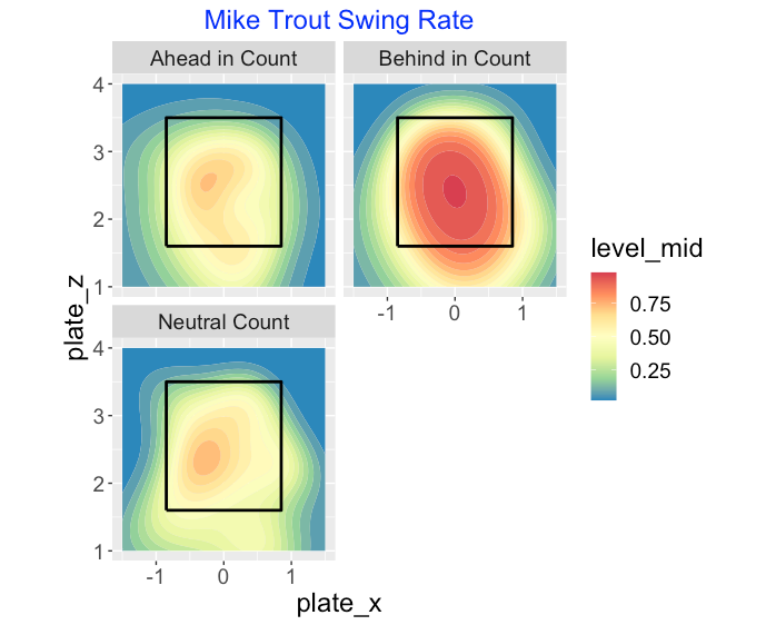
How does Trout’s swing probability depend on the count? I break down the count into three situations (ahead, neutral and behind) and the functions split_count() and swing_contour() are used to construct this graph. We see that Trout rarely swings in ahead in count and neutral count situations. Even in behind in count situations, he only swings at low balls outside of the zone.

Let’s contrast the last graph with a similar display for Jeff McNeil, one of the free swingers. This display is dramatically different. McNeil is very likely to swing in neutral counts and it is likely for him to swing in outside pitches when he is behind in the count.

Making Contact with the Pitch

Let’s revisit our scatterplot and identify nine extreme hitters on their tendency to make contact on a swing.

Here are smoothed estimates of the probability of contact for these nine players. The four low-contact hitters really stand out in this display.

Let’s focus on Luke Voit, who had low contact for the 2019 season. Maybe Voit had problems on a specific pitch type? We breakdown his probability of contact graph by pitch type — fastball or offspeed. We see that Voit missed a lot of high fastballs and low offspeed pitches, even within the zone.

Did Voit struggle against pitchers on a particular side? Being a right-handed hitter, one would expect him to struggle more against right-handed pitcher which seems to be the case here. He misses pitches that are both high and low within the zone. Voit’s behavior against lefties is harder to interpret, although we see that he is likely to miss low in the zone.

Since both pitch type and pitcher side seem to be relevant predictors, it makes sense to graph these probabilities of contact for all combinations of the two predictors. Now we see clearly that Voit struggles against left-handed off-speed pitches inside and low in the zone. He appears most successful on fastballs from left-handers.

Comments

• On my Github Gist site, I have the code for the work on this post. Also this page provides a general introduction to the CalledStrike package.
• The CalledStrike package currently has functions for plotting eleven different metrics as a function of the location in the zone. It would be easy to create functions for new metrics. Since the functions are all pretty short, it would be straightforward to modify the functions for other uses.
• Each of the functions, for example swing_contour(), allows for the input of a single Statcast data frame or a list of several Statcast data frames. By use of the split() function, one can create a list of data frames divided by a grouping variable. When the function has a list argument, it will create a paneled display as shown above
• There are many graphical comparisons possible. One can compare different hitters or pitchers, or a particular hitter across different Statcast seasons. One can see how a particular metric depends on the pitch type, the pitcher side, or the count.
• The package has several “collect” functions that are wrappers to the Statcast scraping functions in Bill Petti’s baseballr package. If one struggles with downloading the Statcast data from Baseball Savant, CalledStrike does include a sample Statcast dataset, sc_example, that one can use to check out the plotting functions.
• Although the CalledStrike package has been improved in some sense, it represents a package in development. So I would appreciate any suggestions for improvement or issues if it exhibits some strange behavior.